Image De-Noising Using a Diffusion Model
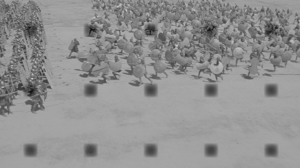
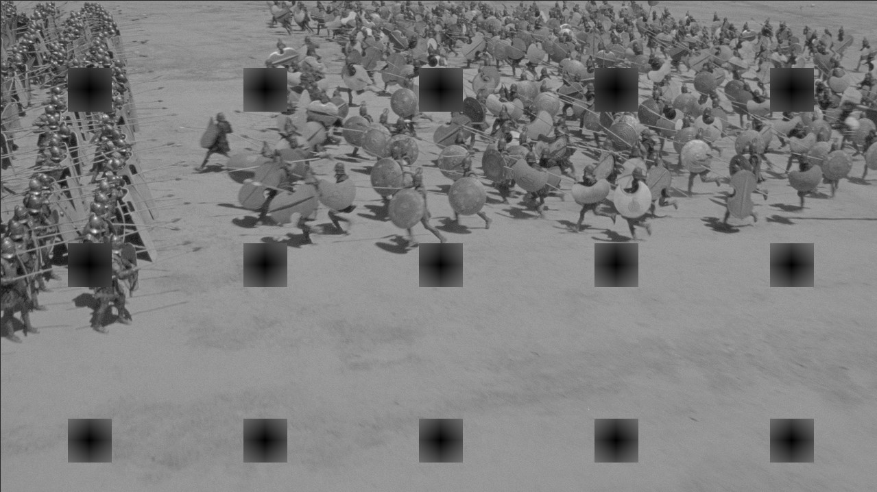
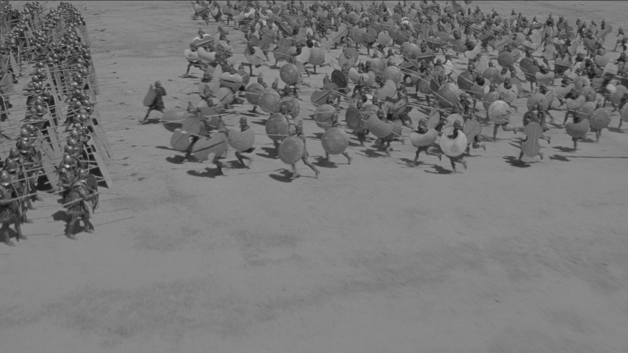
One of the most common problems in cinema is when film degrades or sensors go bad in cameras, the image for certain frames in the film can become corrupted. We want to restore the corrupted image shown below on the left to make it look like the original image on the right. Were this an actual piece of film it would be more appropriate to use video processing techniques which can use the motion of each frame to infer pixel intensity values.
It turns out that for the most part images are quite smooth in terms of brightness (except at object and feature edges). Due to this we can “smooth” out the discontinuous corrupted pixels by using a diffusion model described by the following partial differential equation:
\[\frac{\partial ^ 2 I}{\partial x ^ 2} + \frac{\partial ^ 2 I}{\partial y ^ 2} = f(x,y)\]This model allows brightness to diffuse from one pixel to it’s neighbours creating a smoothly varying image without the discontinuities found in the corrupted image. It should be noted that the diffusivity coefficient has been set to 1 in this case making it a linear isotropic diffusion process. PDEs mainly describe processes in continuous domains and so need to be translated to the discrete domain using the finite difference relationship for partial derivatives. The second order finite difference derivative we need is shown below:
\[\frac{\partial ^ 2 f(x)}{\partial x ^ 2} = \frac{f(x + \Delta x) - 2 f(x) + f(x - \Delta x)}{\Delta x ^ 2} + O(\Delta x ^ 2)\]These can be substituted into the continuous partial differental equation and gives us the discrete form (where $h=\Delta x$):
\[\frac{I[m-1,n] - 2I[m,n] + I[m+1,n]}{h^2} + \frac{I[m,n-1] - 2I[m,n] + I[m,n+1]}{h^2} = f[m,n]\]We can then rearrange this and set $h=1$ as digital images are composed of discrete pixels:
\[I[m-1,n] + I[m+1,n] + I[m,n-1] + I[m,n+1] - 4I[m,n] - f[m,n] = 0\]Further rearranging to obtain $I[m,n]$ by itself yields the pixel update equation we require to obtain the $k+1^{th}$ iteration of the image:
\[I ^ {k+1} [m,n] = \frac{I ^ {k} [m-1,n] + I ^ {k} [m+1,n] + I ^ {k} [m,n-1] + I ^ {k} [m,n+1] - f[m,n] }{4}\] \[E ^ k [m,n] = I ^ {k} [m-1,n] + I ^ {k} [m+1,n] + I ^ {k} [m,n-1] + I ^ {k} [m,n+1] - 4I[m,n] ^ k - f[m,n]\] \[I ^ {k+1} [m,n] = I ^ k [m,n] + \alpha\frac{E ^ k [m,n]}{4}\]This asssignment was originally performed in Matlab but just to improve my coding skills I’ve redone the image processing in Python. First we import the necessary numerical and image processing packages:
# Import all necessary modules
import numpy as np
import pandas as pd
import cv2
from google.colab.patches import cv2_imshow
import scipy.io as sio
import matplotlib.pyplot as pyplot
Next we store the images as NumPy arrays to be operated on with values in the array corresponding to the greyscale value at a pixel site:
# Load original image
original_pic = cv2.imread('greece.tif')

# Load mask for indicating bad pixel sites
bad_pixels = cv2.imread('badpixels.tif', 0) # Note the 0 flag indicates a greyscale image
# Load corrupted picture
mat = sio.loadmat('badpicture.mat')
dataframe = pd.DataFrame(mat.get('badpic'))
I = dataframe.to_numpy()
I = np.double(I)

mat = sio.loadmat('forcing.mat')
dataframe = pd.DataFrame(mat.get('f'))
f = dataframe.to_numpy()
f = np.double(f)
image_iterations = 1000
restored_image = I
E = np.zeros((720, 1280))
alpha = 1
restored_image_error = np.zeros(image_iterations)

for k in range(image_iterations):
  for m in range(1, 719):
    for n in range(1, 1279):
      if bad_pixels[m, n] == 1:
        E[m, n] = restored_image[m - 1, n] + restored_image[m + 1, n] + restored_image[m, n - 1] + restored_image[m, n + 1] - 4 * restored_image[m, n]

        restored_image[m, n] = restored_image[m, n] + alpha * E[m, n] / 4

  restored_image_error_2[k] = (np.abs(restored_image_2 - original_pic)).std(axis=None)
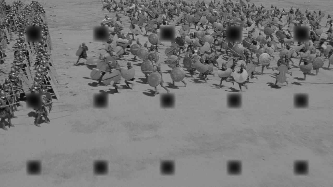
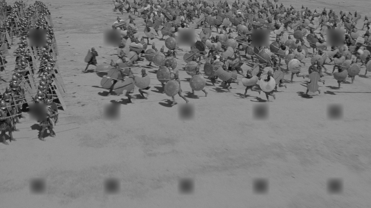
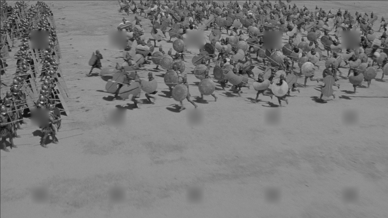
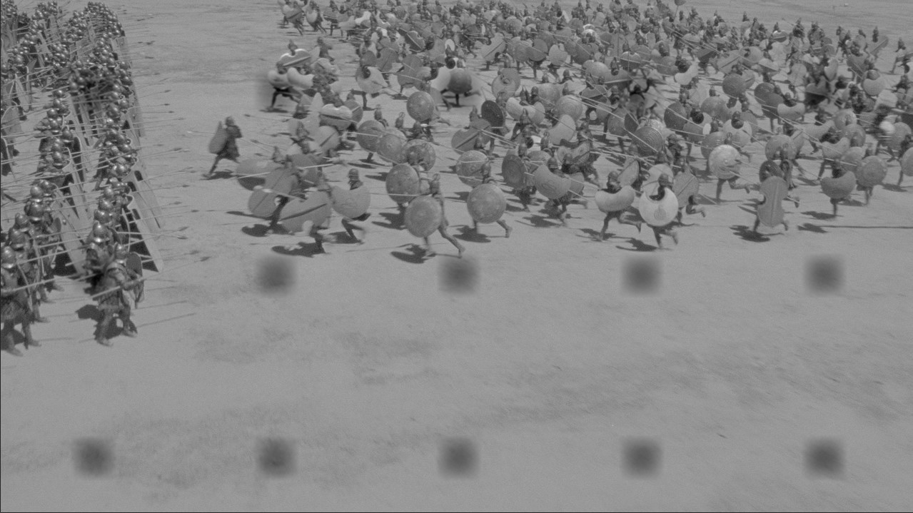
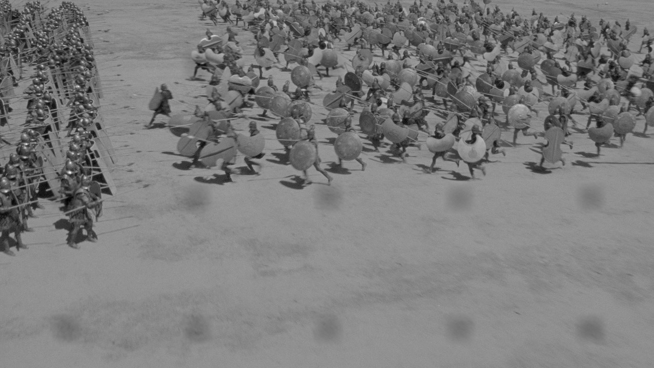
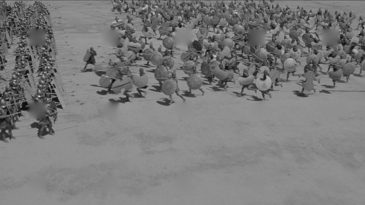
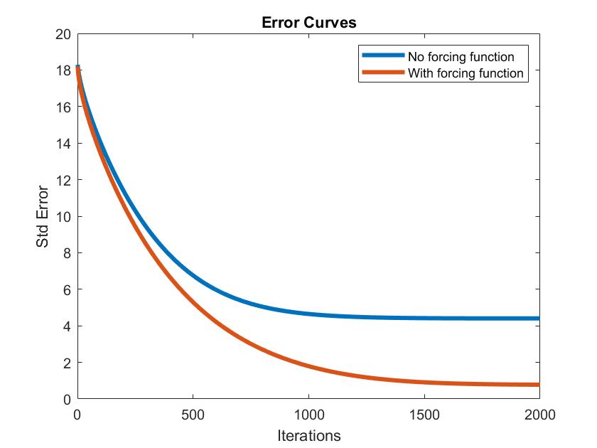
So after 800 iterations while the image does look far better than it was with the giant black rectangles corrupting areas, it appears that the infilled regions with alot of complexity (i.e. the regions over the soldiers) appear extremely blurred. This is due to the. However, we have a trick up our sleeve, we can implement the forcing function we set to zero earlier to enforce a hard boundary around areas we want the algorithm to infill. So what is this forcing function? Well take a look:
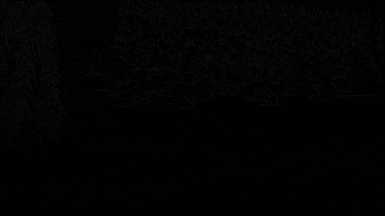
While it is quite hard to make out, this forcing function represents the edges of objects within our image. By enforcing these as restriction on the algorithm, pixel intensity is maintained at these edges thus the algorithm is just filling in and around these boundaries. Our adjusted error function now looks like this:
E[m, n] = restored_image[m - 1, n] + restored_image[m + 1, n] + restored_image[m, n - 1] + restored_image[m, n + 1] - 4 * restored_image[m, n] - f[m, n]
Looking at the results below the forcing function clearly enhances model performance